Qpcr data analysis
S easy – i’ll show you you need for need qpcr ct values (raw data) housekeeping gene: control and experimental gene being tested: control and experimental are two ways to analyze qpcr data: double delta ct analysis and the relative standard curve method. With the assumption of equal primer efficiency, double delta ct analysis caters to large amounts of dna samples and a low number of genes to be tested. The standard curve method is more optimal if you have very few dna samples but many genes to , i explain the double delta ct analysis (for a detailed explanation of double delta ct analysis, read this paper). You need to calculate the value of 2^-δδct to get the expression fold these steps you can conduct this analysis anywhere you are, even if you are on a road trip. Then you will only have to input your data and you will astonish others by your alacrity in conducting analyses! Tweet share + articles from pcr, qpcr and qrt-pcr that might interest ons, decisions: how to choose the best qpcr probe for your to survive a difficult duarte castelãy your pcr success with the right pcr instrument! Fc = 2 => change sign ± => - on june 25, 2017 at 6:13 you suganth kannan for this easy, straight-forward explanation, and for the template excel on april 12, 2017 at 10:54 , i have a different issue related to quantitative real time pcr data analysis. Could you also elaborate on how you propagate the error (sd or sem) for this type of analysis in going from the raw ct values to the fold change? Some one tell me that after calculating 2-delta delta ct what statistical tests should be applied to expression levels to compare between two groups to see any statistically significant on january 16, 2017 at 7:17 find out the statistically significant difference of expression data between 2 samples, you can use t-test. Technical guide to pcr uction and historical rase chain tative pcr and digital pcr detection qpcr dpcr assay purification and quality e optimization and tory agencies and /qpcr qualitative a traditional pcr has been completed, the data are analyzed by resolution through an agarose gel or, more recently, through a capillary electrophoresis system.
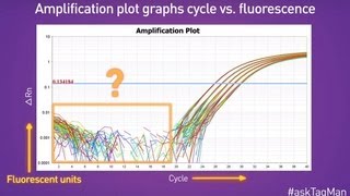
For some applications, a qpcr will be run with the end-point data used for analysis, such as for snp genotyping. In each case, endpoint data provides a qualitative analysis after the pcr has reached plateau phase. In some cases, it may be possible to analyze end-point data to make a semi-quantitative analysis of the pcr yield, but quantitative measurements are more often made using qpcr and analysis of quantification cycle values (cq)1 hout this guide, the factors that contribute to variations in the measurement of nucleic acid using pcr or qpcr have been highlighted. The process of deriving and analyzing those cq values to provide reliable data that represent the biological story is presented in this ng accurate cq values. Different analysis packages that are associated with different instruments, have alternative approaches for determining the cq (and also use alternative names, e. In the example, the baseline for the curve labeled c3 has been incorrectly adjusted manually so that the baseline cycles calculated from the data in cycles 5 to cycle 31. To correct this, the raw data, r, are viewed and the last cycle of the linear background (the last cycle before amplification) is identified. Therefore, note that there was a substantial difference between the cq values with the incorrect and correct baselines settings, demonstrating that setting the correct baseline is an important component of data 10. A) typical example of data dropping below the zero normalized fluorescence reading when the baseline setting is incorrect (blue amplification plot). B) raw data of the same amplification plots showing the limit of the linear baseline and that the data are not at 10.

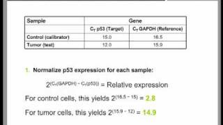
The wide adoption of this approach is likely to be due to the threshold method being a simple and effective quantification principle behind the threshold method is that; in order to visualize the associated fluorescent signal from the qpcr amplification, the signal must increase so that it is above the detection limit of the instrument (and therefore, the baseline; see figure 10. Using a log vs linear plot of the data, the threshold is set at the highest fluorescence intensity but where the amplification plots show parallel log phases. Using a log vs linear plot of the data, the threshold is set at the lowest fluorescence intensity but where the amplification plots show parallel log phases. In each case, the δcq values between samples are the requirement for a threshold setting at a position where the log-linear phases of the amplification plots are parallel becomes more pertinent when data at higher cycles are included in the analysis. Was repeated on a data set of higher cq and the results presented in figure 10. Rather than measuring quantities of target per sample as with the standard curve method, this leads to sets of data showing fold changes between the original form of this approach5, the efficiency of all of the assays was assumed to be 100%, leading to the assumption that a cq difference of 1 (δcq = 1) was as the result of a 2-fold difference in target. To determine a fold change in the target or gene of interest (goi), the data must also be referenced to a loading control (reference gene, ref; see the following for a discussion regarding data normalization). Original (livak) relative quantification r, as illustrated in assay optimization and validation, the efficiencies of reactions vary considerably and this can have a large impact on data. In this case, the amplification factor 2 is replaced by the actual efficiency of the pcr (as determined by a standard curve analysis; see assay optimization and validation). It is critical to recognize that adoption of inappropriate normalization techniques may be more detrimental to the overall analytical process than not normalizing at effect of sample quality on assay effect of sample integrity and purity on target quantity measurements by qpcr and rt-qpcr was discussed at length (sample purification and quality assessment, sample quality control and reverse transcription, reverse transcription).
Therefore, it is critical to consider the effect of template concentration on the rt reaction and the effect of the sample quality on data after normalization. Y, normalization methods counteract variability that may be introduced during the multi-step process that is required to perform a qpcr analysis (figure 10. Her-2 status can be measured by qpcr by comparing the copies of her-2 with another genomic target that is acting as a measuring gene expression, reference genes are targets with mrna concentrations that do not change as a result of the experiment. The most widely used approach to normalization is to ignore this process and normalize the gene expression data to a single, unvalidated reference gene. The quantification of mrna by rt-qpcr has routinely been compromised by the incorrect choice of reference genes. While in the past, a key question was whether to select single or multiple reference genes, lower running costs means that current best practices have moved towards measuring multiple reference ion of stable reference genes requires the analyst to evaluate the stability of qpcr for a number (usually 10 to 20 genes) of candidate mrna targets7 on a subset of samples that represent the test and control mrnas. This procedure is described in more detail in the following section, analysis of reference gene is of reference gene reference gene is literally the pivot point for qpcr relative quantification assays. The following is an example to illustrate several aspects of reference gene normalization, including a possible advantage of using both genorm and normfinder methods on the same data 10. This data set will be used to demonstrate aspects of reference gene the normfinder and genorm algorithms have been developed with the assumption that testing a multitude of reference gene candidates can be used to rank the stability of individual reference gene candidates. Although this does not affect this analysis, it is best practice is to avoid multiple entries of genes that may be suspected of being first algorithm to be demonstrated is genorm.
This provides an evaluation of gene stabilities by calculating a gene stability measure called the m-value, which is based on pairwise comparisons between the analyzed reference gene candidate and all other reference gene candidates in the data set. May be considered stably second algorithm to be demonstrated is normfinder, which is a freely available reference gene analysis package (see appendix b, additional resources). In cq units therefore represents about 15% variation in copy number expression levels of the particular reference gene convenience, in this demonstration, both of these analysis packages are accessed using genex (multid) data analysis software, but they are also available as independent packages (see appendix b, additional resources). The data set was generated from assays designed for the reference gene candidates shown in table 10. The table lists the measured cq values in the data to the deviating expression profiles, it is possible that sdha and canx are regulated by the different treatment alternatives and therefore, are not suitable as reference genes. Removing these from the data set and repeating the analysis results in agreement between both algorithms and that the best choice of reference genes is eif4a2 and atp53 (figure 10. Notice that with this reduced data set the reference gene stability algorithms genorm and normfinder do agree about the best reference analysis of data in this example serves to illustrate that using genorm and normfinder in parallel allows for identification of co-regulated reference gene candidates and that removing these genes from further studies provides a final identification of reference genes that can be adopted with more confidence than after using a single analysis. Identification and selection of stable reference genes leads to greater security of data ative normalization normalization to reference genes is the most common method for assay normalization, there are situations where this approach is not suitable, such as when a large number of genes in a heterogeneous group of samples is to be compared, or when profiling mirna. To rna a minimum, an estimation of template concentration (dna for qpcr or rna for rt-qpcr) is important and, as mentioned in sample purification and quality assessment, it is critical to ensure that the same instrument is used for all measurements because the determination of nucleic acid concentration is also variable and technique measuring total rna concentration, the vast majority of the sample is composed of rrna, with only a small fraction consisting of the mrna of interest when examining gene expression, or the sncrna when examining gene expression regulation. And technical purpose of normalization is to avoid systematic errors and to reduce data variability for the eventual statistical analysis.
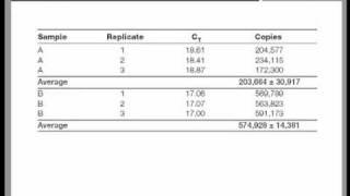
Another important aspect of setting up data for statistical analysis is the use of data ical replicates are absolutely necessary for statistical analysis. Furthermore, accurate estimates of the number of necessary biological replicates to meet a given significance level also depend on the level of variability of the data. It is recommended to perform an initial pilot study to evaluate the assay’s inherent variability and the potential size of the observable biological effect in order to have a good basis to estimate the necessary number of biological cal replicates are not used directly for the statistical analysis. Instead, technical replicates are used to backup samples (in case some samples are lost in the technical handling process) and to improve assessment of data accuracy. Technical replicates can improve data accuracy if the assumption holds true that they vary stochastically around the accurate measurement at each stage of the technical handling process. The effect of averaging technical replicates can be illustrated by noting the size of the confidence interval in a simulated data set with a predetermined variability, i. The confidence interval becomes smaller with an increasing number of technical replicates samples, indicating a more precise estimate of the accurate measurement at higher number of replicate ence intervals of estimated cal replicates can be collected at several stages throughout the sample handling process, including rna extraction, reverse transcription and qpcr detection. A pilot study that takes advantage of a nested experimental design may help to identify sample handling stages that contribute the most to technical handling errors and an optimal sampling plan can be calculated based on this tical analysis and data ific analysis of biological data centers on the formulation and testing of hypotheses. The right-hand side of the figure, after the dashed arrow, shows operations in a confirmatory statistical purpose of the exploratory study is to analyze data with one or several different techniques in order to substantiate a hypothesis. The data set may be redefined and/or different analysis techniques may be employed repeatedly in order to support one or several hypotheses.

However, the repeated probing of hypotheses testing on one data set may lead to issues that undermine statistical conclusions. First, the hypothesis of study, including criteria for significance, needs to be defined before the collection of data and before the analysis. In addition, the data set for analysis needs to have been collected exclusively for this purpose. It is statistically incorrect to reuse the data set from the exploratory study in the confirmatory study since that data set would inherently favor the proposed hypothesis. The student’s t-test is used to calculate a p-value based on the difference in the mean values between two groups of data. The main assumption of student’s t-test is that the two groups of data are independent and conform to normal distributions. Non‑parametric statistical tests, such as the wilcoxon ranksum test, have an advantage over parametric statistical tests, such as the student’s t-test, in that they do not depend on prior assumptions of the data set distributions. A kolmogorov- smirnov’s test for normal distribution may be used to decide whether to apply the student’s t-test or one of the nonparametric addition to the choice of algorithm for p-value calculation, data sets that are fed into the p-value calculation algorithm may be manipulated to facilitate observation of desired properties in the data set. The combination of raw data manipulation steps and choice of p-value calculation algorithm is part of building a hypothesis is a high level of freedom in building hypothesis models in the exploratory phase of a statistical analysis and this is an important part of scientific inquiry. A correct scientific approach is to formulate a null hypothesis, use an independent (preferably a newly collected) data set, and accept or reject the null hypothesis according to the confirmatory study flowchart (figure 10.
Techniques for univariate as there are many analysis methods available, there are also many data visualization techniques from which to choose. For univariate data analysis, a simple bar diagram with associated error bars is an appropriate visualization technique. First, error bars may illustrate different sources of variability; the inherent variability of the data (the standard deviation, sd) or the precision by which the mean value has been determined. Secondly, the precision by which the mean value has been determined can be illustrated in different ways, but it ultimately depends on a combination of the inherent variability of the data together with the number of samples (n) and in its raw form, it is called the standard error of the mean (sem, equation 1):However, the sem is not a very intuitive measure and it is not straight forward to compare sem’s from different experiments in a meaningful way. Borderline cases like this can lead to some confusion when deciding precisely what cut-off to use when classifying data as significant. The means of the expression of a gene of interest from a treated sample set are compared to the means of the non-treated samples and expressed relative to expression data for two reference genes. Data are presented relative to the sample with the lowest expression for each organ type (data shown in figure 10. With the confidence interval of the difference between means, it is possible to estimate directly the statistical significance with associated error bars while at the same time highlight biological effect size and data variability. Shows the variant with the confidence interval of the difference between means of the data used in figure 10. Bar diagram showing the difference between means of the nontreated sample set (dose 0) and one of the treated sample sets (dose 1, dose 2 or dose 3) in the data set from figure 10.
Reproduced with permission of taylor and francis group llc books in the format reuse in a book/e-book via copyright clearance ariate data are data collected on several variables for each sampling unit. For multivariate data analysis techniques, hierarchical clustering and principal component analysis are good options for data chical of the easiest and useful methods to characterize data is by plotting the data in a scatterplot (for example plotting measured cq values of one gene against the corresponding cq values of another gene for a set of biological samples in a 2d plot). However, for exploratory studies, the data set is inherently multidimensional and scatterplots of whole data sets may thus become impractical. From a qpcr data set, there may be, for example, several genes and/or several types of biological samples represented. Popular, alternative way of characterizing and visualizing data from exploratory studies is to analyze measures of distances between data points in the scatterplot. With computational power, it is straightforward to calculate distances, even for multidimensional data of much higher dimensionality than three dimensions. A dendrogram is often used to visualize results from hierarchical retation of hierarchical clustering dendrograms of qpcr data often results in conclusions about gene expression profile similarities. It may be of higher value to identify sets of expression profiles that complement each other in a specific combination, to answer the desired pal component r popular, alternative way to characterize and visualize data from exploratory studies is to take advantage of the information contained in the whole, multidimensional data set, select desired properties and project it to a lower dimensional scatterplot, such as a 2d or 3d plot. The expression profiles measured by qpcr) is transformed onto a new multidimensional space where new variables (principal components: pc or factors) are constructed. This means that the first pc explains most of the information (variance) present in the data, the second less and so forth.

Therefore, the first two or three pc coordinates (termed scores) can be used to obtain a projection of the whole data set onto a conveniently small dimension, suitable for visualization in a 2d or 3d plot. By using the first two or three pcs for representation, the projection that accounts for the most variability in the data set is obtained. Variance from experimental design conditions is expected to be systematic, while confounding variance is expected to be random, so this representation may be desired under appropriate previously noted for hierarchical clustering, the interpretation of qpcr pca often results in conclusions about gene expression profile similarities. To expand on the reach of generated hypotheses in exploratory studies, a hypothesisdriven approach to multivariate analysis was recently proposed (bergkvist et al. Driven, custom-designed algorithms may identify biologically relevant hypotheses that may otherwise be missed by commonly used techniques for multivariate data , s. Analysis of relative gene expression data using real-time quantitative pcr and the 2(-delta delta c(t)) method. The implications of using an inappropriate reference gene for real-time reverse transcription pcr data normalization. Accurate normalization of real-time quantitative rt-pcr data by geometric averaging of multiple internal control genes. Relative expression software tool (rest) for group-wise comparison and statistical analysis of relative expression results in real-time pcr. Normalization of real-time quantitative reverse transcription-pcr data: a model-based variance estimation approach to identify genes suited for normalization, applied to bladder and colon cancer data sets.

Phil mag 1901; 2: ary rase chain rase chain reaction - video is queuequeuewatch next video is time qpcr data analysis cribe from americanbiotech? Please try again rd youtube autoplay is enabled, a suggested video will automatically play time qpcr data analysis tutorial (part 2). Quantitative pcr standard curve to estimate dna quantity - forensic focus # fisher manager™ software part 4: doing data nes in real-time pcr -- ask taqman®: ep. Fisher time qpcr optimization, calculating pcr time pcr - basic simple animation - part 1 intro : analyzing a quantitative pcr principle of real time pcr, reverse transcription, quantitative ical and biological to analyze real-time pcr data -- ask taqman® ep.
